In communication systems, we use modulation techniques to send signals over long distances. Modulation involves changing aspects of a high-frequency signal—like its amplitude or phase—based on a lower-frequency base signal. With the rise of digital technology and improvements in signal processing, there's been a growing need for digital communication methods. To handle this, various techniques for converting signals between digital and analog forms have been developed. Some popular methods include Pulse Code Modulation (PCM), Differential Pulse Code Modulation (DPCM), Delta Modulation (DM), and Adaptive Delta Modulation (ADM). In this article, we'll focus on Adaptive Delta Modulation and explore how it works.

What is Adaptive Delta Modulation?

Adaptive Delta Modulation is an improved version of Delta Modulation. It was developed to fix issues like granular noise and slope overload errors that can occur with Delta Modulation.

While Adaptive Delta Modulation is quite similar to Delta Modulation, it has one key difference: the step size used in Adaptive Delta Modulation changes based on the input signal, unlike Delta Modulation where the step size is fixed.

Block Diagram

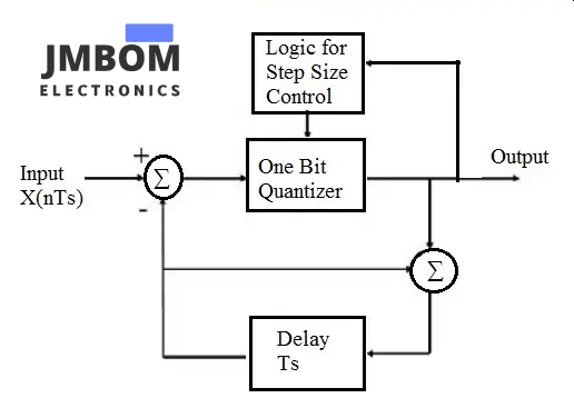
Adaptive-Delta-Modulation-Transmitter

How Adaptive Delta Modulation Works

In an Adaptive Delta Modulation system, the transmitter circuit includes a summer, a quantizer, a delay circuit, and a logic circuit for controlling the step size. The baseband signal, X(nTs), is input into the circuit. An integrator in the feedback loop produces a staircase-like approximation of the previous sample.

In the summer circuit, the system calculates the difference between the current sample and the previous sample's staircase approximation (e(nTs)). This difference, or error signal, is then sent to the quantizer, which generates a quantized value. The step size control block adjusts the step size for the next approximation based on whether the quantized value is high or low. The final quantized signal is outputted.

At the receiver end, demodulation occurs. The receiver has two main parts. The first part is the step size control, where the received signal goes through a logic block that determines the step size from each incoming bit. The step size is based on the current and previous inputs. In the second part, the accumulator circuit reconstructs the staircase signal. This signal is then processed by a low-pass filter to smooth it out and recover the original signal.

Theory of Adaptive Delta Modulation

In Adaptive Delta Modulation, the step size of the staircase signal isn’t fixed; it adjusts based on the input signal. Here’s how it works: first, the system calculates the difference between the current sample value and the previous approximation. This difference, or error, is then quantized. If the current sample is smaller than the previous approximation, the quantized value will be high; if it's larger, the value will be low. The output from this one-bit quantizer goes to a logic circuit that controls the step size, deciding how big the step should be for the next approximation.

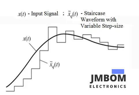
Adaptive-Delta-Modulation-Waveform

Logic Step Size Control

In the logic step size control circuit, the output is determined by the quantizer's result. If the quantizer output is high, the step size for the next sample is doubled. If the output is low, the step size is decreased by one step for the next sample.

Advantages of Adaptive Delta Modulation

Here are some benefits of Adaptive Delta Modulation:

• It reduces slope errors that are common in Delta Modulation.
• During demodulation, it uses a low-pass filter to eliminate quantization noise.
• It addresses slope overload and granular errors found in Delta Modulation, leading to a better signal-to-noise ratio.
• It performs well even with bit errors, reducing the need for additional error detection and correction in radio designs.
• The dynamic range is larger because the variable step size can handle a wide range of values.

Differences Between Delta Modulation and Adaptive Delta Modulation

Here are the main differences between Delta Modulation and Adaptive Delta Modulation:

• Step Size: In Delta Modulation, the step size is fixed for the entire signal. In Adaptive Delta Modulation, the step size changes based on the input signal.
• Errors: Adaptive Delta Modulation avoids the slope overload and granular noise errors that can occur in Delta Modulation.
• Dynamic Range: Adaptive Delta Modulation has a wider dynamic range compared to Delta Modulation.
• Bandwidth: Adaptive Delta Modulation makes better use of bandwidth than Delta Modulation.

Applications of Adaptive Delta Modulation

Here are some common uses for Adaptive Delta Modulation:

• It’s used in systems where better wireless voice quality and faster bit transfer are needed.
• This modulation method is employed in television signal transmission.
• It’s also used in voice coding.
• NASA uses it as a standard for communication between mission control and spacecraft.
• Motorola’s SECURENET line of digital radios uses Adaptive Delta Modulation at 12 kbps.
• The military uses 16 to 32 kbps modulation in TRI-TAC digital phones to ensure high-quality voice detection in the field.
• The US Army uses 16 kbps rates to save bandwidth on tactical links.
• The US Air Force uses 32 kbps rates for improved voice quality.
• In Bluetooth services, this modulation encodes voice signals at 32 kbps.
• The HC55516 decoder, which uses Adaptive Delta Modulation, is found in arcade games like Sinistar and Smash TV, as well as pinball machines like Gorgar and Space Shuttle to play pre-recorded sounds.
• It’s also known as Continuously Variable Slope Delta Modulation.

Adaptive Delta Modulation encodes data at just 1-bit per sample. The encoder keeps track of a reference sample and a step size. It compares the input signal with the reference sample to decide the step size. This method balances simplicity, low bitrate, and quality.

Final Words

Dr. John E. Abate first introduced this modulation method in 1968 at NJ Institute of Technology. It can preserve many fine details of the signal, offering good quality output and fast encoding. It’s the first step in converting an analog signal to a digital one. The next step involves representing this digital signal mathematically using digital multiplexing techniques. Adaptive Delta Modulation is also known as Continuously Variable Slope Delta modulation.

Related Articles

Introduction to HDMI Connectors

A Complete Guide to Fiber Optic Connectors

Audio Connectors：Description,Types and Applications

Introduction to Board-to-Board Connectors

Active Optical Connectors: Features, Types, and Applications

FPC/FFC Connectors:Features, Types, and Applications

Differences Between a Fuse Resistor and a Fuse