
Introduction of Passive Low Pass Filter
Catalog
Description of Passive Low Pass FilterIdeal Filter Response CurvesThe Low Pass Filter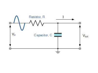 Frequency Response of a 1st-order Low Pass Filter
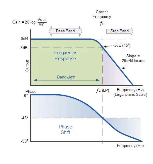 Passive Low Pass Filter Gain at ƒcLow Pass Filter SummaryApplications of Passive Low Pass Filters
Description of Passive Low Pass Filter
A Low Pass Filter is a circuit designed to tweak, reshape, or block unwanted high frequencies from an electrical signal. It only lets through the signals that the circuit designer wants.
Passive Low Pass Filter
Passive RC filters work by filtering out the signals, letting only those sinusoidal input signals through based on their frequency. The simplest of these is the passive low pass filter network.For low-frequency applications (up to 100kHz), we usually build passive filters using basic RC (resistor-capacitor) networks. But when we’re dealing with higher frequencies (over 100 kHz), we typically use RLC (Resistor-Inductor-Capacitor) components.
Passive filters consist of passive components like resistors, capacitors, and inductors. They don’t have any amplifying elements like transistors or op-amps, which means they don’t boost the signal. So, the output level is always lower than the input.Filters are named based on the frequency range of signals they let through while blocking or “attenuating” the others. The most common filter designs include:
The Low Pass Filter – This filter lets low frequency signals from 0Hz up to its cut-off frequency, ƒc, pass through, but it blocks any signals that are higher.
The High Pass Filter – On the flip side, this filter only allows high frequency signals starting from its cut-off frequency, ƒc, and going up to infinity. It blocks all the lower frequencies.
The Band Pass Filter – This one lets signals that fall within a specific frequency range between two points pass through, while it blocks both the lower and higher frequencies on either side of that range.
You can create simple first-order passive filters (1st order) by hooking up a single resistor and a single capacitor in series across an input signal (VIN). You take the output of the filter (VOUT) from where those two components connect.
Depending on how you connect the resistor and capacitor for the output signal, you’ll end up with either a Low Pass Filter or a High Pass Filter.
Basically, the job of any filter is to let certain frequency signals pass through unchanged while reducing the strength of all the other unwanted ones. We can define the amplitude response characteristics of an ideal filter using the ideal frequency response curve for the four basic filter types.
Ideal Filter Response Curves
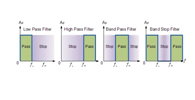
Ideal Filter Response Curves
Filters can be split into two main types: active filters and passive filters. Active filters use amplifying devices to boost the signal strength, while passive filters don’t have any amplifying devices, which means they can’t strengthen the signal. Since passive filters are made up of two passive components, the output signal usually has a smaller amplitude compared to the input signal. So, passive RC filters end up attenuating the signal, giving them a gain of less than one (or unity).
A Low Pass Filter can be created using capacitance, inductance, or resistance. Its job is to really cut down the signal above a certain frequency while allowing little to no attenuation below that frequency. The point where this change happens is called the “cut-off” or “corner” frequency.
The simplest low pass filters are made up of just a resistor and a capacitor. But there are also fancier low pass filters that use a mix of series inductors and parallel capacitors. In this tutorial, we’ll focus on the simplest version: a passive two-component RC low pass filter.
The Low Pass Filter
You can easily make a simple passive RC Low Pass Filter (LPF) by connecting a single resistor and a single capacitor in series, like this: (insert diagram). In this setup, the input signal (VIN) goes to the series combo of the resistor and capacitor, but the output signal (VOUT) is taken from across just the capacitor.
This kind of filter is usually called a “first-order filter” or “one-pole filter.” Why? Because it has only one reactive component—the capacitor—in the circuit.
RC Low Pass Filter Circuit
RC Low Pass Filter Circuit
As we talked about in the Capacitive Reactance tutorial, the reactance of a capacitor changes inversely with frequency, while the resistor’s value stays the same as the frequency shifts. At low frequencies, the capacitive reactance (XC) of the capacitor is much bigger compared to the resistance (R).
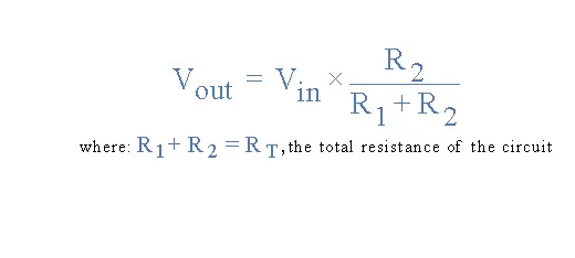
While the circuit above is set up as an RC Low Pass Filter, you can also think of it like a frequency-dependent variable potential divider circuit, kind of like what we went over in the Resistors tutorial. In that tutorial, we used this equation to figure out the output voltage for two resistors connected in series.
We also know that the capacitive reactance of a capacitor in an AC circuit is defined as:
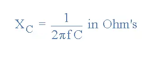
the capacitive reactance of a capacitor in an AC circuit
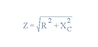
Opposition to current flow in an AC circuit is called impedance (symbol Z). For a series circuit with a single resistor and a single capacitor, we can calculate the circuit impedance like this:
Now, if we plug our impedance equation into the resistive potential divider equation, we get:
RC Potential Divider Equation
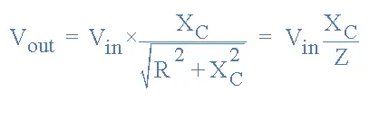
RC Potential Divider Equation
This means the voltage across the capacitor (VC) is way larger than the voltage drop across the resistor (VR). But at high frequencies, it’s the other way around: VC is small and VR is large because of the change in capacitive reactance.
So, by using the potential divider equation for two resistors in series and plugging in the impedance, we can calculate the output voltage of an RC Filter for any given frequency.
Low Pass Filter Example No. 1
Let’s look at a Low Pass Filter circuit with a 4.7kΩ resistor in series with a 47nF capacitor, connected to a 10V sinusoidal supply. We’ll calculate the output voltage (VOUT) at 100Hz and then at 10,000Hz (or 10kHz).
Voltage Output at a Frequency of 100Hz
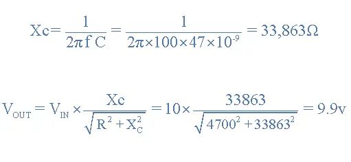
Voltage Output at a Frequency of 100Hz
Voltage Output at a Frequency of 10,000Hz (10kHz).
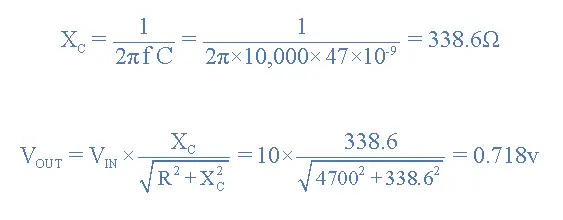
Voltage Output at a Frequency of 10,000Hz (10kHz)
Frequency Response
We can see from the results above, that as the frequency applied to the RC network increases from 100Hz to 10kHz, the voltage dropped across the capacitor and therefore the output voltage ( VOUT ) from the circuit decreases from 9.9v to 0.718v.
By plotting the networks output voltage against different values of input frequency, the Frequency Response Curve or Bode Plot function of the low pass filter circuit can be found, as shown below.
Frequency Response of a 1st-order Low Pass Filter
Frequency Response of a 1st-order Low Pass Filter
The Bode Plot shows the Frequency Response of the filter to be nearly flat for low frequencies and all of the input signal is passed directly to the output, resulting in a gain of nearly 1, called unity, until it reaches its Cut-off Frequency point ( ƒc ). This is because the reactance of the capacitor is high at low frequencies and blocks any current flow through the capacitor.
After this cut-off frequency point the response of the circuit decreases to zero at a slope of -20dB/ Decade or (-6dB/Octave) “roll-off”. Note that the angle of the slope, this -20dB/ Decade roll-off will always be the same for any RC combination.
Any high frequency signals applied to the low pass filter circuit above this cut-off frequency point will become greatly attenuated, that is they rapidly decrease. This happens because at very high frequencies the reactance of the capacitor becomes so low that it gives the effect of a short circuit condition on the output terminals resulting in zero output.
Then by carefully selecting the correct resistor-capacitor combination, we can create a RC circuit that allows a range of frequencies below a certain value to pass through the circuit unaffected while any frequencies applied to the circuit above this cut-off point to be attenuated, creating what is commonly called a Low Pass Filter.
For this type of “Low Pass Filter” circuit, all the frequencies below this cut-off, ƒc point that are unaltered with little or no attenuation and are said to be in the filters Pass band zone. This pass band zone also represents the Bandwidth of the filter. Any signal frequencies above this point cut-off point are generally said to be in the filters Stop band zone and they will be greatly attenuated.
This “Cut-off”, “Corner” or “Breakpoint” frequency is defined as being the frequency point where the capacitive reactance and resistance are equal, R = Xc = 4k7Ω. When this occurs the output signal is attenuated to 70.7% of the input signal value or -3dB (20 log (Vout/Vin)) of the input. Although R = Xc, the output is not half of the input signal. This is because it is equal to the vector sum of the two and is therefore 0.707 of the input.
As the filter contains a capacitor, the Phase Angle ( Φ ) of the output signal LAGS behind that of the input and at the -3dB cut-off frequency ( ƒc ) is -45o out of phase. This is due to the time taken to charge the plates of the capacitor as the input voltage changes, resulting in the output voltage (the voltage across the capacitor) “lagging” behind that of the input signal. The higher the input frequency applied to the filter the more the capacitor lags and the circuit becomes more and more “out of phase”.
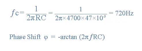
The cut-off frequency point and phase shift angle can be found by using the following equation:
Cut-off Frequency and Phase Shift
Cut-off Frequency and Phase Shift
For our simple example of a “Low Pass Filter” circuit, the cut-off frequency (ƒc) is 720Hz, with the output voltage being 70.7% of the input voltage value and a phase shift angle of -45°.
Second-order Low Pass Filter
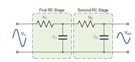
So far, we’ve seen that simple first-order RC low pass filters are made by connecting a single resistor in series with a single capacitor. This single-pole setup gives us a roll-off slope of -20dB/decade for frequencies above the cut-off point at ƒ-3dB. However, if that -20dB/decade (-6dB/octave) slope isn’t enough to get rid of unwanted signals, we can use two stages of filtering, like this:
Second-order Low Pass Filter
Second-order Low Pass Filter
In the circuit above, we’ve got two passive first-order low pass filters connected together, which forms a second-order or two-pole filter network. This means we can turn a first-order low pass filter into a second-order one just by adding another RC network. The more RC stages we add, the higher the order of the filter.
If we cascade (or connect) n number of RC stages, we call the resulting circuit an “nth-order” filter, and it has a roll-off slope of “n x -20dB/decade.”
For example, a second-order filter would have a slope of -40dB/decade (-12dB/octave), and a fourth-order filter would have a slope of -80dB/decade (-24dB/octave). This means that as we increase the filter order, the roll-off slope gets steeper, making the stop band response approach its ideal characteristics.
Second-order filters are really important and commonly used in filter designs because we can combine them with first-order filters to create higher-order filters. For instance, a third-order low-pass filter can be made by cascading a first-order and a second-order low pass filter.
But there’s a downside to cascading RC filter stages. While there’s no limit to how many filter orders we can create, as the order goes up, the gain and accuracy of the final filter tend to decline.
When identical RC filter stages are connected together, the output gain at the desired cut-off frequency (ƒc) gets reduced (attenuated) depending on how many stages we’ve used, as the roll-off slope increases. We can define the amount of attenuation at the cut-off frequency using this formula:
Passive Low Pass Filter Gain at ƒc
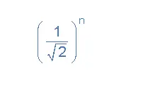
Passive Low Pass Filter Gain at ƒc
where “n” is the number of filter stages.
For a second-order passive low pass filter, the gain at the corner frequency (ƒc) will be equal to 0.7071 x 0.7071 = 0.5Vin (-6dB). For a third-order passive low pass filter, it’ll be 0.353Vin (-9dB), and for a fourth-order, it’ll be 0.25Vin (-12dB), and so on. The corner frequency (ƒc) for a second-order passive low pass filter is determined by the resistor-capacitor (RC) combination and is given as:
2nd-Order Filter Corner Frequency
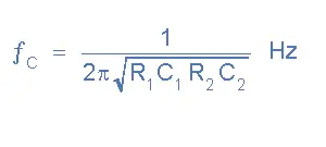
2nd-Order Filter Corner Frequency
In reality, as the filter order increases, the -3dB corner frequency point of the low pass filter—and thus its pass band frequency—shifts from its original calculated value. This change is determined by the following equation:
2nd-Order Low Pass Filter -3dB Frequency
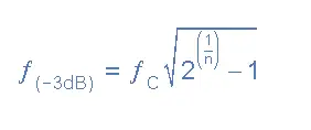
2nd-Order Low Pass Filter -3dB Frequency
where ƒc is the calculated cut-off frequency, n is the filter order, and ƒ-3dB is the new -3dB pass band frequency due to the increase in filter order.
The frequency response (Bode plot) for a second-order low pass filter, assuming the same -3dB cut-off point, would look like this:
Frequency Response of a 2nd-order Low Pass Filter
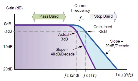
Frequency Response of a 2nd-order Low Pass Filter
In practice, cascading passive filters to create higher-order filters can be tricky because the dynamic impedance of each filter affects its neighboring network. To reduce the loading effect, we can make the impedance of each following stage 10 times that of the previous stage, so R2 = 10 x R1 and C2 = 1/10th of C1. Second-order filters and higher are usually found in the feedback circuits of op-amps, which are often called Active Filters or used as phase-shift networks in RC Oscillator circuits.
Low Pass Filter Summary
To sum it all up, the Low Pass Filter has a constant output voltage from DC (0Hz) up to a specific cut-off frequency (ƒC). This cut-off frequency point corresponds to 0.707 or -3dB (where dB = -20 log(VOUT/VIN)) of the voltage gain that’s allowed to pass.
The frequency range below this cut-off point (ƒC) is known as the Pass Band since the input signal can pass through the filter. In contrast, the frequency range above this cut-off point is called the Stop Band because the input signal is blocked from passing through.
A simple first-order low pass filter can be created using a single resistor in series with a single non-polarized capacitor (or any single reactive component) across the input signal Vin, with the output signal Vout taken across the capacitor.
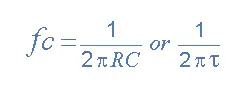
You can find the cut-off frequency or -3dB point using the standard formula, ƒc = 1/(2πRC). The phase angle of the output signal at ƒc is -45° for a Low Pass Filter.
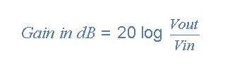
The gain of the filter, or any filter really, is usually expressed in decibels and is a function of the output value divided by its corresponding input value, given by:
Applications of Passive Low Pass Filters
You’ll find passive low pass filters in audio amplifiers and speaker systems, where they help direct lower frequency bass signals to larger bass speakers or reduce high-frequency noise, like that annoying “hiss.” In these audio applications, a low pass filter is sometimes called a “high-cut” or “treble cut” filter.
If we switch the positions of the resistor and capacitor so that the output voltage is taken across the resistor, we’d create a circuit that has an output frequency response curve similar to a high pass filter, which we’ll dive into in the next tutorial.
Time Constant
So far, we’ve focused on the frequency response of a low pass filter when it’s dealing with sinusoidal waveforms. We’ve seen that the cut-off frequency (ƒc) depends on the resistance (R) and capacitance (C) in the circuit, and adjusting either component changes the cut-off frequency.
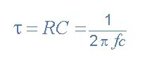
We also know that the phase shift of the circuit lags behind the input signal due to the time it takes to charge and discharge the capacitor as the sine wave changes. This combination of R and C creates a charging and discharging effect on the capacitor, which is called its Time Constant (τ). This gives the filter a response in the time domain.
The time constant, tau (τ), is related to the cut-off frequency ƒc as follows:
Or expressed in terms of the cut-off frequency, ƒc as:
The output voltage (VOUT) depends on the time constant and the frequency of the input signal. With a smooth, sinusoidal signal, the circuit behaves like a simple first-order low pass filter, as we’ve seen.
But what happens if we switch the input signal to a “square wave” with a sharp “ON/OFF” type of shape? The output response would change dramatically, resulting in a circuit commonly known as an Integrator.
The RC Integrator
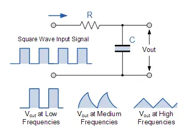
The Integrator is basically a low pass filter working in the time domain that converts a square wave “step” input signal into a triangular waveform output as the capacitor charges and discharges. A triangular waveform consists of alternating, equal positive and negative ramps.
As shown below, if the RC time constant is long compared to the input waveform’s time period, the output waveform will be triangular in shape. The higher the input frequency, the lower the output amplitude compared to the input.
The RC Integrator Circuit
The RC Integrator Circuit
This makes this type of circuit perfect for converting one type of electronic signal to another, which is super useful in wave-generating or wave-shaping circuits.

Christopher Anderson
Christopher Anderson has a Ph.D. in electrical engineering, focusing on power electronics. He’s been a Senior member of the IEEE Power Electronics Society since 2021. Right now, he works with the KPR Institute of Engineering and Technology in the U.S. He also writes detailed, top-notch articles about power electronics for business-to-business electronics platforms.
Subscribe to JMBom Electronics !